Introduction to the vector space model
Introduction

To put it briefly, the vector space model is an algebraic model that represents text as a vector: each component reflects how important a term is, and whether or not it appears (a bag of words) in a document.
In this model, text is treated as points in an n-dimensional Euclidean space, where each dimension corresponds to one term in the vocabulary. The i-th component of a document vector counts how often the i-th term appears in that document. Similarity between two documents is defined either as the distance between those points or as the angle between the vectors.
Each term in the vector space carries a weight. Many weighting schemes exist, but tf–idf (term frequency–inverse document frequency) is a common way to score and rank a term within a document. MySQL full-text search uses this idea too. In essence, tf–idf is a ranking function that turns raw text into a vector space model via those weights. The vector space model and tf–idf were developed by Gerard Salton in the early 1960s.
Simple as it is, the vector space model and its variants remain a standard way to represent text in data mining and information retrieval. One weakness is high dimensionality: in a web search engine the space can easily reach tens of millions of dimensions.
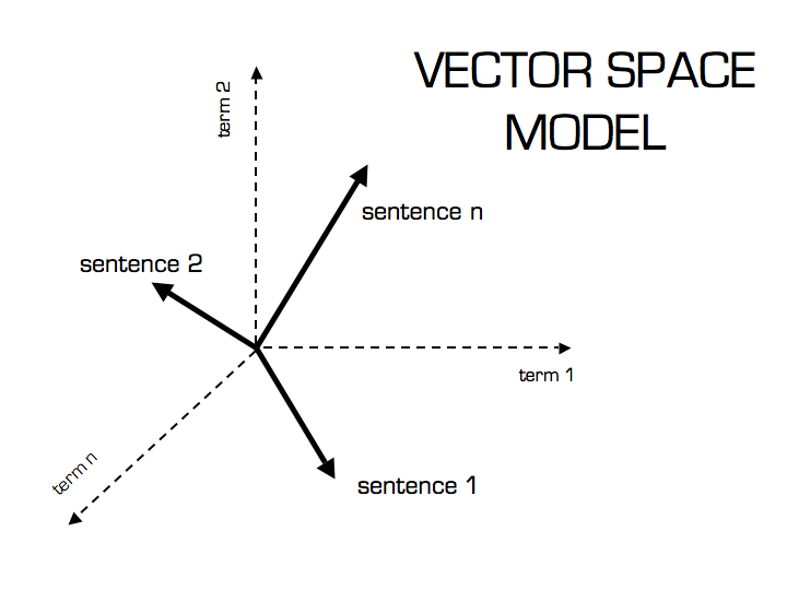 Illustration by Christian S. Perone
Representing text as vectors and term frequency
Example:
The first row lists Shakespeare plays. The first column lists terms, and the cells show whether each term appears in each play (binary presence).
| Anthony and Cleopatra | Julius Caesar | The Tempest | Hamlet | Othello | Macbeth | |
|---|---|---|---|---|---|---|
| Anthony | 1 | 1 | 0 | 0 | 0 | 1 |
| Brutus | 1 | 1 | 0 | 1 | 0 | 0 |
| Caesar | 1 | 1 | 0 | 1 | 0 | 1 |
| Calpurnia | 0 | 1 | 0 | 0 | 1 | 0 |
| Cleopatra | 1 | 0 | 0 | 0 | 0 | 0 |
| Mercy | 1 | 0 | 1 | 1 | 1 | 1 |
| Worser | 1 | 0 | 1 | 1 | 1 | 0 |
Binary incidence matrix (Introduction to Information Retrieval)
Each document is then a vector—for example, Julius Caesar is
$$\begin{bmatrix} 1 \ 1 \ 1 \ 1 \ 0 \ 0 \ 0 \end{bmatrix}$$
The cells can instead show how many times each term appears in each play. That is term frequency.
| Anthony and Cleopatra | Julius Caesar | The Tempest | Hamlet | Othello | Macbeth | |
|---|---|---|---|---|---|---|
| Anthony | 157 | 73 | 0 | 0 | 0 | 1 |
| Brutus | 4 | 157 | 0 | 2 | 0 | 0 |
| Caesar | 232 | 227 | 0 | 2 | 0 | 1 |
| Calpurnia | 0 | 19 | 0 | 0 | 1 | 0 |
| Cleopatra | 57 | 0 | 0 | 0 | 0 | 0 |
| Mercy | 2 | 0 | 3 | 8 | 5 | 8 |
| Worser | 2 | 0 | 1 | 1 | 1 | 0 |
Here each document (each play, in this case) is a count vector. For example, Julius Caesar is
$$\begin{bmatrix} 73 \ 157 \ 227 \ 19 \ 0 \ 0 \ 0 \end{bmatrix}$$
Term frequency \(\mathit{tf}_{t,d}\) counts how often term \(t\) appears in document \(d\). Raw counts alone are not enough.
If a term appears ten times in one document and once in another, the first document is more relevant—but not ten times more relevant. Relevance does not scale linearly with raw term frequency.
Log-frequency weighting
The log-frequency weight of term \(t\) in document \(d\) is:
$$w_{t,d} = 1 + \log(\mathit{tf}_{t,d})$$
when \(\mathit{tf}_{t,d} > 0\); otherwise \(w_{t,d} = 0\).
If the term does not appear, \(\mathit{tf}_{t,d} = 0\). Because \(\log(0)\) is undefined (and tends to \(-\infty\)), we add \(1\) in the formula.
If the term appears in the document:
- once → \(w = 1\)
- twice → \(w \approx 1.3\)
- ten times → \(w = 2\)
- a thousand times → \(w = 4\)
The score for a document–query pair is the sum of weights for terms that appear in both the query and the document:
$$\sum_{t \in q \cap d} \bigl(1 + \log(\mathit{tf}_{t,d})\bigr)$$
The score is zero if none of the query terms appear in the document.
Inverse document frequency (idf)
Rare terms matter more than terms that show up everywhere. Every language has high-frequency, low-information words (in English: a, the, to, of, …); in full-text search these are often called stop words.
With raw term frequency, more occurrences mean a higher score and rare terms get pushed down—yet rare terms often carry more information than common ones, so we need a different treatment.
In a collection of documents about the auto industry, the word “car” might appear in almost every document. To limit that effect and improve relevance between query and document, we down-weight terms with high document frequency: take the total number of documents \(N\) and divide by the number of documents in which the term appears.
Let \(\mathit{df}_t\) be the number of documents that contain term \(t\). Smaller \(\mathit{df}_t\) (relative to \(N\)) means the term is more discriminative.
We define the idf weight of term \(t\) as:
$$\mathrm{idf}_t = \log_{10}!\left(\frac{N}{\mathit{df}_t}\right)$$
We use \(\log_{10}(N/\mathit{df}_t)\) instead of \(N/\mathit{df}_t\) alone so idf does not explode—again, raw frequency is not the same as semantic importance.
In MySQL’s internals this is sometimes expressed as \(\log_{10}!\left(\frac{N - n_f}{n_f}\right)\) (see the manual).
(More on MySQL full-text internals)
How idf affects ranking
For a single-keyword query, idf does not change the ordering of documents; it mainly helps separate relevant from irrelevant material. idf changes ranking when the query has at least two terms. For example, for the query “capricious person”, idf makes capricious count for more in the final ranking than person, because person is far more common.
Collection frequency vs document frequency
| term | dtf | idft |
|---|---|---|
| calpurnia | 1 | log(1000000/1)=6 |
| animal | 100 | log(1000000/100)=4 |
| sunday | 1,000 | 3 |
| fly | 10,000 | 2 |
| under | 100,000 | 1 |
| the | 1,000,000 | 0 |
Collection frequency of term \(t\) is how often \(t\) appears across the whole collection. The table is an idf example with \(N = 10^{6}\): each term gets a corresponding idf. Document frequency is how many documents contain term \(t\).
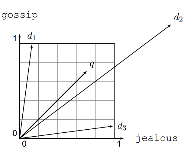
The query as a vector
To search for a phrase in a collection (full-text query), we compare that query to each document. The idea is to treat the query as a vector too (as above) and rank documents by how close they are to the query vector.
Documents that are closer to the query get higher scores.
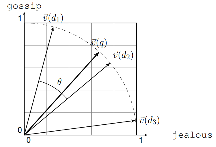
We can compare two vectors by Euclidean distance or by the angle between them. Distance has a drawback: it can be large for vectors of different lengths even when the relative word distributions match—for example, if document \(d’\) is simply document \(d\) duplicated.
The Euclidean distance between \(\vec{q}\) and \(\vec{d}_2\) can be large even when the term distributions in \(\vec{q}\) and \(\vec{d}_2\) are very similar.
In the figure, you can see that the distance between \(\vec{q}\) and \(\vec{d}_2\) is sizable even though the term distributions in query \(\vec{q}\) and document \(\vec{d}_2\) are quite alike.
So in vector space we care more about the angle than about the distance between points.
Using angle instead of distance
As a thought experiment, take a document \(d\) and append a copy of itself to get \(d’\). Semantically the content is the same. Then \(\vec{d}^{\prime}\) has twice the length of \(\vec{d}\) but the same direction as \(\vec{d}\).
Yet the Euclidean distance between \(d\) and \(d’\) is large, even though the content is identical.
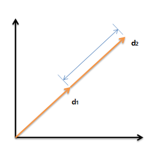
So instead of ranking by Euclidean distance, we rank by the angle between the document vector and the query vector.
Larger angle → lower cosine and lower score. When the angle is 0, the score is maximal (\(= 1\)).
Two equivalent ways to say it:
- Rank documents by increasing angle between query and document
- Rank documents by decreasing cosine between query and document
Documents are ranked by decreasing cosine similarity:
- \(\cos(\vec{d}, \vec{q}) = 1\) when \(\vec{d}\) and \(\vec{q}\) align
- \(\cos(\vec{d}, \vec{q}) = 0\) when document \(\vec{d}\) and query \(\vec{q}\) share no terms
Why normalize document length?
Longer documents tend to have:
- higher term frequencies—the same word can appear more often simply because there is more text;
- more distinct terms, which increases overlap with the query by chance.
Cosine normalization reduces the bias of long documents versus short ones. A vector can be length-normalized by dividing each component by the vector’s length. Length is computed with the L2 norm:
$$\lVert \vec{x} \rVert = \sqrt{\sum_i x_i^2}$$
For \(\vec{d}\):
$$\begin{bmatrix} 3 \ 4 \end{bmatrix}$$
we have \(\lVert \vec{d} \rVert = \sqrt{3^2 + 4^2} = 5\).
For \(\vec{d}’\):
$$\begin{bmatrix} 6 \ 8 \end{bmatrix}$$
we have \(\lVert \vec{d}’ \rVert = \sqrt{6^2 + 8^2} = 10\).
Dividing a vector by its L2 norm yields a unit-length vector (unit vector).
The Euclidean distance between the two vectors is large even though the angle is the same. After normalizing \(d\) and \(d’\), both become
$$\begin{bmatrix} 0.6 \ 0.8 \end{bmatrix}$$
—identical. Long and short documents become comparable after normalization.
That still is not a complete fix, which is why people also use pivoted document length normalization.
Cosine similarity
$$\cos(\vec{q}, \vec{d}) = \frac{\vec{q} \cdot \vec{d}}{\lVert \vec{q} \rVert , \lVert \vec{d} \rVert} = \frac{\vec{q}}{\lVert \vec{q} \rVert} \cdot \frac{\vec{d}}{\lVert \vec{d} \rVert} = \frac{\sum_{i=1}^{\lvert V \rvert} q_i d_i}{\sqrt{\sum_{i=1}^{\lvert V \rvert} q_i^2} ; \sqrt{\sum_{i=1}^{\lvert V \rvert} d_i^2}}$$
- \(q_i\) is the tf–idf weight of term \(i\) in the query.
- \(d_i\) is the tf–idf weight of term \(i\) in the document.
- \(\cos(\vec{q}, \vec{d})\) is the cosine similarity between \(\vec{q}\) and \(\vec{d}\)—the cosine of the angle between them.
For length-normalized vectors, cosine similarity is just the dot product:
$$\cos(\vec{q}, \vec{d}) = \vec{q} \cdot \vec{d} = \sum_{i=1}^{\lvert V \rvert} q_i d_i \qquad \text{for } \vec{q}, \vec{d} \text{ length-normalized}$$
For turning the ideas above into code, see: Short introduction to the vector space model
References
- Christopher D. Manning, Prabhakar Raghavan & Hinrich Schütze, Introduction to Information Retrieval (2008), http://nlp.stanford.edu/IR-book/html/htmledition/irbook.html
- Christian S. Perone, “Machine learning: text feature extraction (tf–idf), part I” (2011), http://pyevolve.sourceforge.net/wordpress/?p=1589
- Nguyễn Tuấn Đăng, Khai mỏ văn bản tiếng Việt với bản đồ tự tổ chức (2002) — thesis (Vietnamese), PDF